Revisiting Fibonacci Sequence

Functional Equations #

One evening, I felt down for no reason. I felt like not doing anything I could do, including consuming content. Then came a flash of thought, “It’s been a while you have involved yourself with Functional Equations”. This was the spark moment that led me to a short journey of a surge of inspiration from the infinite abyss of artistic temperament.

I, at once, googled for worksheets on Functional Equations and I was presented with a good amount of those. I started solving them one by one until I saw this one:

$$ f(n)=f(n-1)+f(n-2) $$ At first sight, I recognized it to be a functional equation representing the Fibonacci Series. However, from my experience in teaching programming, I know how to use this to generate the nth number of the series using looping and recursion statements. Never have I given it a thought to have a simple function representation. In fact, if it has one(and it has one), we can write a program that runs with \(O(c)\) algorithmic complexity. This represents the fastest runtime for any algorithm. The algorithmic complexities being \(O(n)\) and \(O\left(\phi^n\right)\) with \(\phi\) being golden ratio \((\phi=(1+\sqrt{5}) / 2\) ) for looping and recursion respectively, this function will outmatch the two algorithms I have been teaching my students for a long while. Hence, I started the attempt to solve the functional equation representing the Fibonacci Sequence. After a minute, I came up with the following:

We consider the solution of the form

$$ f(n)=\beta^n \text { for some } \beta \in \mathbb{R} $$ Now, we have $$ \beta^n=\beta^{n-1}+\beta^{n-2} $$ from which we conclude that $$ \beta^2=\beta+1 $$ solving for this quadratic equation, we get two distinct roots: $$ \beta_1=\frac{1+\sqrt{5}}{2}, \beta_2=\frac{1-\sqrt{5}}{2} $$ A general solution of the sequence can be written as:

$$ f(n)=c_1\left(\frac{1+\sqrt{5}}{2}\right)^n+c_2\left(\frac{1-\sqrt{5}}{2}\right)^n $$ where \(c_1, c_2\) are coefficients to be determined by the initial values given in the problem statement. The initialvalues are: \(f(0)=0, f(1)=1\). Using the intital conditions, we have: $$ c_1+c_2=0 $$ $$ c_1\left(\frac{1+\sqrt{5}}{2}\right)+c_2\left(\frac{1-\sqrt{5}}{2}\right)=1 $$ This is a system of linear equations in two variables and we have multiple methods to solve them. Using any one of them will yield us:

$$ c_1=\frac{1}{\sqrt{5}}, c_2=-\frac{1}{\sqrt{5}} $$ Thus,

$$ f(n)=\frac{1}{\sqrt{5}}\left\{\left(\frac{1+\sqrt{5}}{2}\right)^n-\left(\frac{1-\sqrt{5}}{2}\right)^n \right \} $$

Programming the Fibonacci Sequence #

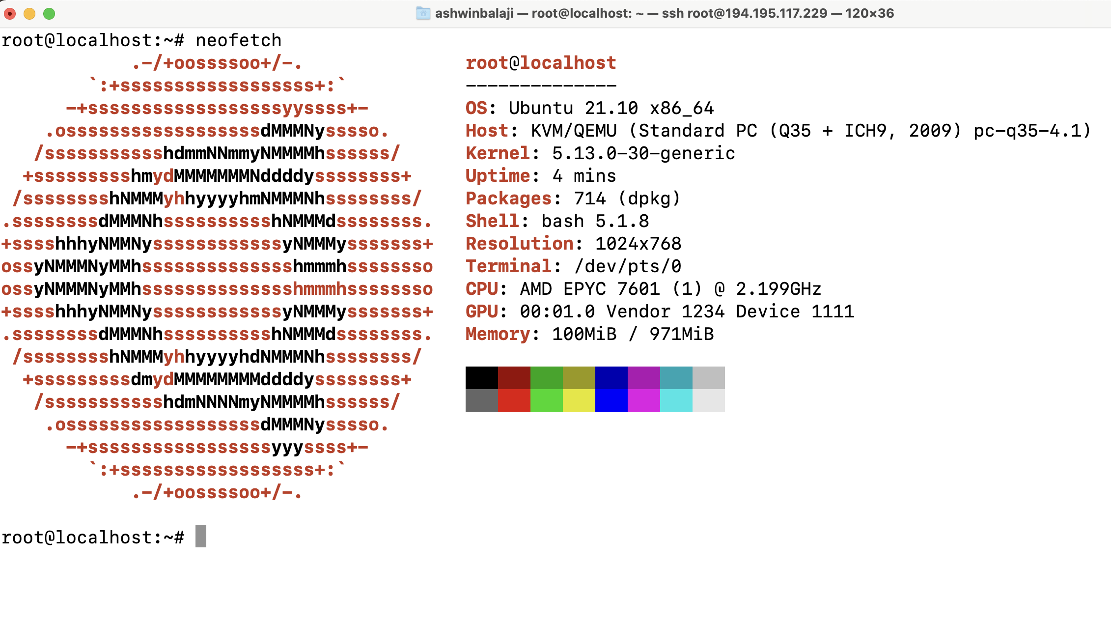
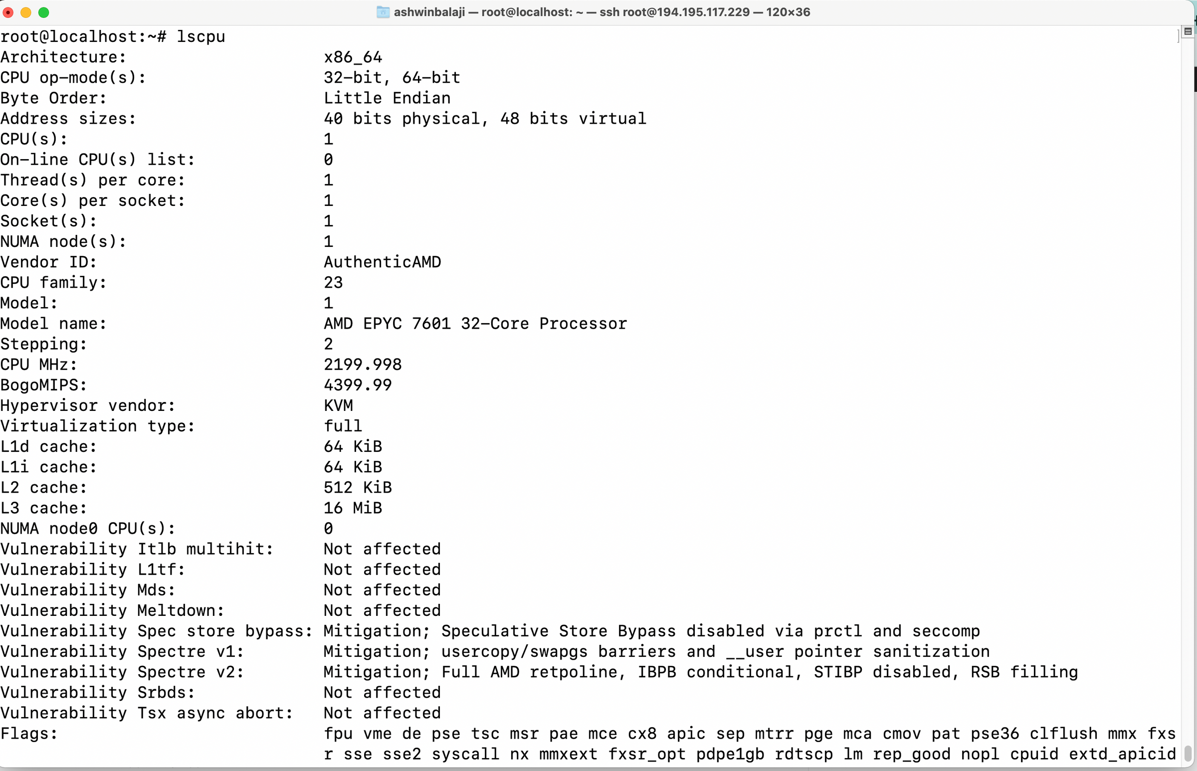
Now let us put this stuff to testing in the programming environment. I chose to create a new Ubuntu virtual machine in Linode(not a sponsor) with 1 vCPU and 1GB of RAM to make the test as fair and square as possible. Here is the spec of the machine I used for testing:

Code used to Run the below programs:

Benchmarks and Remarks #

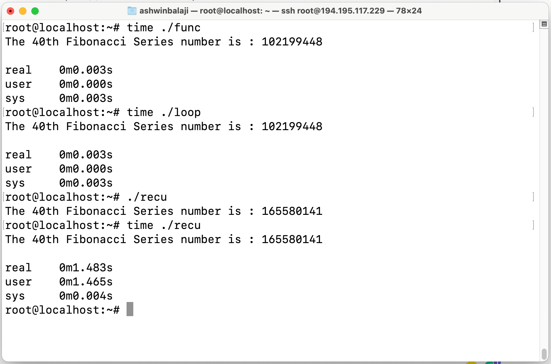
The recursion, as expected, has taken the longest time as predicted by the Big - O notation from the algorithmic analysis. However, we couldn’t see the difference in performance between function implementation and the looping implementation. That depends upon how efficient the pow(a, b) function is implemented within C++ 11 and we hit a bottleneck where the upper limit of int datatype is reached faster and the further positive numbers turn out to be negative by the nature of how the negative numbers are represented in the computers. Also, due to the differences in initial conditions in the program, we see different results for different algorithms that can be calibrated easily. However, we can see that the difference in runtime will scale pretty quickly when we discuss simulations in the scales of Quantum Chromodynamics where we use lattice gauges to study the strong interactions’ non-perturbative regimes. Hence, the requirement to optimize the programs as much as possible. This simple example is single-threaded and doesn’t deal with concurrency. When we add heterogeneous computing to our mix, we have huge possibilities for optimizations.